Open the file Sales and Expenses and save as Net Profit
Insert Rows
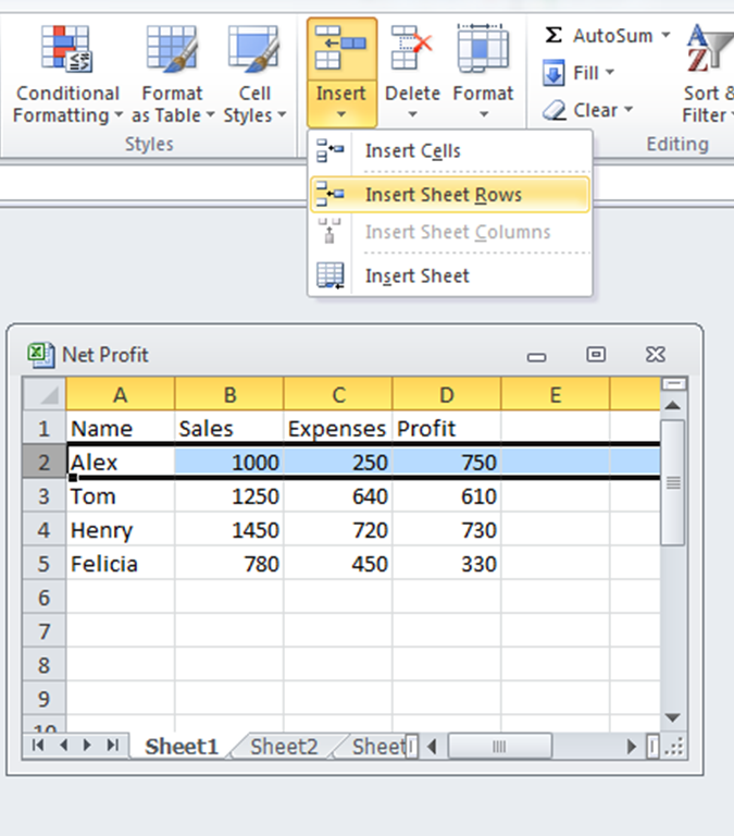
To select a row 2, click the mouse at row numbered 2.
Click Insert icon and choose Insert Sheet Rows.
Excel will insert a new row at row 2.
Type the following:
At cell E1 – Tax
F1 – Net Profit
E2 – 7%
To calculate Tax at 7% for Alex, in cell E3, type the formula =D3*E2 and press Enter.
Place the pointer in cell E3 and copy down the formula till cell E6.
Hmm…. Something is not right!
Let us find out what happened.
Place the pointer in cell E4 and look at the Formula Bar.
It displays =D4*E3.
D4 has the profit, but E3 does not have 7%. Right?
Why this has happened?
Whenever you copy a formula down, row numbers in the formula will increase.
While this is OK for column D (profit), the tax rate 7% is only at cell E3 and should not be changed.
So how we can fix this?
$E$2 (absolute cell address) is to keep the cell fixed, while you copy a formula so it always refers to 7%.
To calculate Net Profit for Alex, in cell F3, type the formula =D3 – E3 and press Enter.
Place the pointer in cell F3 and copy down the formula till cell F6.
Type the following:
Save the file.
Use the formatting tool bar and try to format the spreadsheet as follows.
Insert Rows
To select a row 2, click the mouse at row numbered 2.
Click Insert icon and choose Insert Sheet Rows.
Excel will insert a new row at row 2.
Type the following:
At cell E1 – Tax
F1 – Net Profit
E2 – 7%
To calculate Tax at 7% for Alex, in cell E3, type the formula =D3*E2 and press Enter.
Place the pointer in cell E3 and copy down the formula till cell E6.
Hmm…. Something is not right!
Let us find out what happened.
Place the pointer in cell E4 and look at the Formula Bar.
It displays =D4*E3.
D4 has the profit, but E3 does not have 7%. Right?
Why this has happened?
Whenever you copy a formula down, row numbers in the formula will increase.
While this is OK for column D (profit), the tax rate 7% is only at cell E3 and should not be changed.
So how we can fix this?
- First, select cells E3 to E6 and press Delete button.
- Now in cell E3, type the formula =D3*$E$2 and press Enter.
- Place the pointer in cell E3 and copy down the formula till cell E6.
$E$2 (absolute cell address) is to keep the cell fixed, while you copy a formula so it always refers to 7%.
To calculate Net Profit for Alex, in cell F3, type the formula =D3 – E3 and press Enter.
Place the pointer in cell F3 and copy down the formula till cell F6.
Type the following:
- At cell A9 – Total
- To find total sales at B9, type =sum(B4:B5) and Press Enter.
- Place the pointer in cell B9 and copy the formula to the right till cell F6.
Save the file.
Use the formatting tool bar and try to format the spreadsheet as follows.


